Lab8: Los Angeles Fire of 2009

In August of 2009, a wildfire known as the Station wildfire broke out and set the Los Angeles County into a state of emergency. With flames reaching “300 to 400 feet” (Los Angeles Times), it is considered the largest wildfire in LA County’s modern history. It burned 160,557 Acres of the Los Angeles National Forest, destroying 209 structures and took 647 personnel to contain (Inciweb – 9640). Communities of La Canada-Flintridge, La Crescenta, Acton, Soledad Canyon, Pasadena and Glendale were evacuated due to the fire (Inciweb – 9360).The cost of fighting the fire was around $83.1 million (KTLA).

After reading reports, I became curious on why the fire was so difficult to handle. After some research, it was revealed that the fact that this was not a ‘wind driven’ fire was what made this fire special. Instead, the topography and the makeup of dry brush caused this extreme fire behavior. The “unusual mix of fuel, from chaparral and dry grass at lower elevations to pine at higher ones, coupled with record heat and slopes that are among the steepest of any mountain range in the country” (The New York Times) created a different type of fire than the wind driven fires that firefighters are more accustomed to handle.

I decided to examine for myself the linkage between the fuel distribution and the spread of fire for the Station Fire. The first map, a reference map, provided shows the extent of the Station Fire regarding the location in LA County. It is clear that, by the distribution of roads and highways, this fire burned quickly and fiercely in the mostly non-populated area of the LA County. The area is also very much in a higher mountain range as the digital elevation model demonstrates. The topology of the region would have made it very inaccessible for the firefighters to haul their equipment into as well as having so much variation in the height making it a difficult terrain to fight fires on.

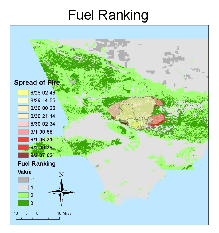
Using the Fuel Ranking data from the California Department of Forestry, I created a Fuel Ranking map and overlayed the spread of fire by time on top of it. First thing to notice is that most of the area underneath the area burned has a rank of 3, and the rest has a rank of 2. With higher ranked fuels having more energy to burn, it is evident that the fire followed this pattern by engulfing the fuel rich areas. Looking at the spread of the fire by time on top of the fuel ranking provides more insight into where the fire chose to spread. The fires started at the south part of the total areas burned and quickly spread north towards the directions of higher fuel rankings. This direct correlation was what the reports were referring to as the dry chaparral that fueled the fire instead of wind.

Because of this non wind driven fire, “L.A. County Fire and Forest Services said they would change their procedures so that both agencies would immediately fight to extinguish any fire in the southern portion of the Angeles National Forest so that future fires don't become as massive and dangerous as the Station Fire.” (KTLA) As it can be observed in the maps I created, the Station fire served as a very costly reminder that the fire can be just as much damaging without the presence of the wind.

Archibold, Randal. (2 September 2009). “California Fire Is Pushed Back.” The New York Times. Web. 13 June. 2012. http://www.nytimes.com/2009/09/03/us/03fires.html?_r=1

Bloomekatz, Ari B. (2 September 2009). “Station fire is largest in L.A. County's modern history.” Los Angeles Times. Web. 13 June. 2012. http://latimesblogs.latimes.com/lanow/2009/09/station-fire-is-largest-in-la-county-history.html

"Station Fire Evening Update Aug. 31, 2009." inciweb.org. Web. 13 June. 2012. http://inciweb.org/incident/article/9360/

“Station Fire Update Sept. 27, 2009.” Inciweb.org. Web. 13 June. 2012. http://inciweb.org/incident/article/9640/

(2 October 2009). “Report: Number of Firefighters Reduced Before Station Fire.” KTLA News. Web. 13 June. 2012. http://www.ktla.com/news/landing/ktla-angeles-fire,0,5292469.story

Lab 7

This map shows clearly the distribution of Black population in the US by county. It is very evident that there are a lot of black concentrated counties in the South compared to the rest of the country. There are counties with less than 1 percent reported black population that there is no data available (represented by white). The history of the black population in United States is reflected in current day’s population distribution.

The percentage of Asian population by county is shown in the map. Even the most concentrated counties have less than 50% of the population identified as Asian. Because the West coast is closer to Asia through the Pacific Ocean, it is logical that many of them settled on the West coast such as California and Washington. Especially because of the shorter history of immigration compared to other races, the spread of the Asian population into the rest of the continental US is low, with the exception of couple major cities such as New York.

The Other Races population percentage map shows the races not classified as follows: "White", "Black or African American", "American Indian and Alaska Native", "Asian" and "Native Hawaiian and Other Pacific Islander". From the look of the distribution, an educated guess can be made that this mostly consists of Hispanic population in the United States. Many of the counties near the US/Mexico border have higher percentage of “other races” while counties further North have lower percentages. Again, with the exception of major places such as Tristate area and Florida, the rest of the continental US has low spread of the ‘other races’ population.

The census map series and the experience with ArcGIS have been very beneficial. It was very interesting to visualize the data that I grabbed from an outside source, convert it into tables, joining them with the shape data in order to make meaning out of the data. The maps I created clearly show the distribution of population for specific races. From that, I could make inferences and search for the reason behind that, connecting it back to history. I think this lab was very useful in practicing working with data tables and analyzing the data in a different way that I could not do with just an excel file. It really showed the power of GIS that was not allowed without the geographic data.